Reprojecting a raster invents values
Reprojecting a set of coordinates is exact. Every point goes through the inverse of one map and the forward of another, and nothing is lost that was not already lost to floating point.
Reprojecting a picture is not, and the reason has nothing to do with the projections.
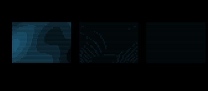
What a warp actually does
A raster is a grid of samples, and warping it means producing a different grid of samples of the same thing. The operation runs backwards, and the backwardness is the first thing worth explaining because it is not obvious.
Forward mapping — take each source cell, project its centre into the target, deposit the value — leaves holes where the target grid is coarser than the image of the source, and piles several values into one cell where it is finer. The output is not a raster; it is a scatter.
Inverse mapping — take each target cell centre, carry it back through the target’s inverse and the source’s forward map, and read the source grid at that position — produces exactly one value per target cell, always. Every warping routine does this, and it means the projections are evaluated in the direction opposite to the one the data is moving.
The reading is the problem. That position is not a source cell centre; it falls somewhere inside a source cell, and a value has to be produced for it from the neighbours. That is the whole of the loss, and it would happen with no projection at all if the two grids were merely offset.
The control: a warp that should change nothing
Before measuring a loss, the machinery has to be shown not to be producing one. Warping the raster into the projection it is already in and back gives an RMS departure of — floating-point noise on values of order one.
That check earns its place. Every part of the pipeline is exercised — the target grid’s extent, the inverse map, the interpolation, the return trip — and the only thing that is not is the projection’s difference. So a bug in the grid bookkeeping, an off-by-half in the cell centres, or an inverted axis would show here, on a case whose answer is known exactly.
The three kernels, and what separates them
The kernels are usually compared with adjectives: nearest is blocky, bilinear is smooth, cubic is sharper. What actually separates them is an order of convergence — refine the grid and the error falls as the cell size to some power — and the power is a number that can be measured and can be wrong.
Warping into an azimuthal equal-area projection and back, on rasters from 48 × 32 to 160 × 110 cells, with the RMS departure from the field measured on the grid it started on:
| kernel | RMS at 90 × 60 | fitted order |
|---|---|---|
| nearest | 1.13 × 10⁻² | 1.004 |
| bilinear | 6.29 × 10⁻⁴ | 1.983 |
| Catmull–Rom cubic | 2.71 × 10⁻⁶ | 2.930 |
First, second and third order, fitted from the refinement rather than quoted from the formulae, and the site’s gate holds each to within 0.15 of its integer. That is the difference between the three stated as a property: halving the cell size halves nearest’s error, quarters bilinear’s, and divides the cubic’s by eight.
The absolute numbers matter too. At a realistic raster size the cubic is four thousand times closer to the underlying field than nearest-neighbour is, which is a larger gap than the adjectives suggest.

The claim that had to be withdrawn
The first version of this essay’s assertion said something else, and recording why it failed is more useful than the claim would have been.
The intended argument was a trade: bilinear is closer to the field on average and pays for it in contrast, because smoothing removes extremes. That would have been a satisfying pairing — accuracy against sharpness, each kernel winning one — and the check was written as bilinear loses more of the field’s variance than nearest does.
It passed at one grid size and failed at the next. Measured across five:
| cells | bilinear variance lost | nearest variance lost |
|---|---|---|
| 48 × 32 | 0.634% | 0.102% |
| 64 × 44 | 0.341% | 0.459% |
| 90 × 60 | 0.178% | 0.024% |
| 120 × 80 | 0.101% | 0.045% |
| 160 × 110 | 0.055% | 0.004% |
Bilinear’s loss is systematic — it falls smoothly at every refinement, which is what a filter does. Nearest’s is erratic in size and in sign, because nearest-neighbour is not a filter at all: it moves values without changing them, so what it does to the variance depends on which cells happen to be duplicated and which dropped.
So the trade is real and the quantity was wrong. What nearest gives up is not contrast, it is position: every value is genuine and is in the wrong place by up to half a cell, which is exactly the quantisation the pixel is a place with a size measures for a vertex. What bilinear gives up is that no output value is a value that was ever measured.
The surviving assertion is the one that can be checked: bilinear’s variance loss must fall at every refinement. Nearest’s is not asserted, because it does not do anything monotone and asserting that it does was the mistake.
The case where the choice is forced
For a continuous field the kernels are a trade. For a categorical raster — land cover, soil class, an administrative code — there is no trade at all.
Averaging two class numbers produces a third class number that means something else. Interpolating between class 3 and class 7 gives 5, which is neither and is a real category with a real meaning. So a categorical raster must be resampled by nearest-neighbour, accepting first-order positional error, because every higher-order kernel is a weighted mean and a weighted mean of labels is nonsense.
That is a clean instance of the field’s rule that the operation decides the method, and it is one of the few places where the right answer is forced rather than balanced. It also means a pipeline that warps a mixed dataset has to know which of its layers are measurements and which are labels — information that is not in the raster, and which is exactly the kind of thing a coordinate without its system is not a location is about, one level up.
The other half of the loss: cells are not the same size
Interpolation is the visible half of a warp. The other half is that a target cell and the source cells it draws from cover different amounts of ground, and by a factor that varies across the picture — which is the areal scale factor, the same quantity computing an area needs a surface measures at 3.06 over a mid-latitude cell.
Where the target grid is coarser than the source, a target cell covers several source cells and reading a single interpolated value throws the rest away. Point sampling a signal that has been undersampled is aliasing, and the repair is to average over the cells the target cell actually covers — which is a different operation from interpolation and is why serious resampling distinguishes magnifying from minifying.
Where it is finer, the target has more cells than the source has information, and every kernel is inventing detail. The picture gets larger and no sharper, which is the honest description of what an upsampled raster is.
A warp between projections is usually both at once, in different parts of the same image, because the areal factor varies: an equal-area target from a conformal source is minifying at high latitude and magnifying near the equator. One warp, two regimes, and a single kernel choice applied to both — which is a limitation of the operation as it is universally implemented rather than of any particular implementation.
What decides which regime a point is in is the ratio of the two planes’ areal factors there, and that ratio varies by a factor of three across a single mid-latitude picture on the planes this essay warps between.

Every warp is another one
The loss compounds, which is why the operational advice is stronger than the per-warp numbers suggest.
Each round trip applies the interpolation again, so a dataset warped from its native projection to a working one, to a display one, and back for storage has been resampled three times, and the errors do not cancel — the second warp cannot know what the first removed. For bilinear the variance loss accumulates in the same direction at every pass, because a low-pass filter applied twice is a narrower low-pass filter.
Hence the rule everybody who handles imagery arrives at independently: reproject once, from the original, to whatever is finally needed. Not because a warp is expensive but because it is lossy, and because the loss is a property of the number of warps rather than of the distance between the projections.
That is a sharper statement than it looks. The distance between projections barely matters — the loss comes from grid misalignment, which is nearly as bad for two similar projections as for two different ones. A warp between two systems that differ by a few metres loses almost as much as a warp across the world.
Where this differs from everything else in the field
The rest of this field is about operations that give a wrong answer to a well-posed question: an area that is three times too large, a neighbour that is the wrong site, a segment 718 kilometres from its route. Each of those has a right answer that a better method reaches.
A raster warp does not. There is no correct value for a target cell whose centre falls between source samples: the information was never collected, and every kernel is a different way of admitting that. The best available method converges to the underlying field as the grid is refined, which is precisely the statement that the answer depends on the sampling rather than on the arithmetic.
That places it beside the site’s other genuinely irreducible results rather than beside its measurable errors. No map is faithful is a theorem about surfaces; the antimeridian is a cut in the numbers is a fact about circles; this is a fact about samples, and it is the reason a picture is a different kind of object from a set of coordinates.
What the tiling scheme does with all this
The screen half of this field is the largest consumer of raster warping there is. Imagery is captured in a sensor’s own geometry, orthorectified onto a projection, and served in the tiling’s — which is at least one warp and usually two, at every zoom level, for the whole world.
Two consequences follow from the numbers above. The kernel choice is a policy with a measurable cost, and at continental zoom levels where a pixel is hundreds of metres the resampling error is small against the ground resolution — the reason nobody notices. And the pyramid is not a stack of independent warps: a level is built by downsampling the level below, so the deepest level is warped once and the shallow ones are filtered repeatedly, which is why a zoomed-out tile is smoother than the ground it represents rather than merely coarser.
A screen map is a pyramid of tiles has the scheme; the connection here is that the pyramid’s exact halving, which makes the geometry free, does not make the resampling free.
It is also why the kernel choice is usually made by default. At the zoom levels where imagery is served the cell is tens or hundreds of metres of ground, and a first-order kernel’s half-cell displacement is below anything a reader could see — so a decision with a four-thousandfold spread in accuracy is taken by whichever library was reached for.
The asymmetry with vector data, which is the field’s cleanest contrast
Two datasets covering the same ground, reprojected by the same transformation: the coordinates survive it exactly and the picture does not. That asymmetry is worth stating plainly because it decides how each kind of data should be stored.
Vector geometry is closed under reprojection. A point maps to a point, exactly; the file is the same size afterwards; the operation is invertible to floating-point noise. What changes is what straight means between the vertices — a straight segment is a claim about a plane measures that at 718 kilometres over an ocean — and densifying along the geodesic removes even that, at a known cost in vertices.
A raster is not. Its samples are welded to a grid, the grid is a property of a plane, and changing the plane means new samples. There is no densification that fixes it, because the missing information is not between the stored vertices — it is not stored at all.
The storage advice follows directly and differs for the two. Keep vector data in whatever plane suits its consumers, densified along the ground; a consumer reprojecting it loses nothing. Keep raster data in the plane it was captured in, warp on demand, and never store the result — because every stored warp is a source that has already been resampled once, and the next consumer will resample it again.
What the measurement rests on
One last note on method, because the field this raster carries is not an image.
It is an analytic function — a sum of two sinusoids in longitude and latitude — sampled onto the grid. That is deliberate and it is the same decision as the coastline refusal at foundation: a photograph has a sharpening history and a compression history, and the error of an interpolation measured on one is partly a measurement of those. Here the truth is known at every point exactly, so the RMS is the kernel’s error and nothing else, and the convergence orders come out at their theoretical values because there is nothing else in the signal to disturb them.
The cost of that choice is honesty about what has not been measured: real imagery has edges, and an edge is where interpolation kernels differ most and where convergence orders stop applying. What is measured here is the smooth case, which is the case the orders are defined for, and the site says so rather than implying the numbers cover everything.
Why never store the warp is advice nobody takes, and what to do instead
The storage rule above is correct and it is also unusable as stated, because warping is expensive and a raster served to a thousand readers cannot be warped a thousand times. So the rule is broken in every production system, and it is worth saying what the honest compromise is rather than pretending it is not.
Store the recipe, not the result. A virtual raster — a small file naming the source, the source’s own plane, the target plane and the kernel, resolved at read time — is the warp expressed as a description rather than as pixels. The reader who wants the target plane gets it; the reader who wants a different target gets one warp from the original rather than two warps in series; and the file records what was done, which pixels never do.
That is not a novel proposal. GDAL’s VRT is exactly this and has been for two decades, and it is used mostly for mosaicking and rescaling rather than for the thing it is best at.
Because the real defect in a stored warp is not the error, it is the silence. A resampled raster looks like a captured one. It has the same header, the same band structure, the same nodata convention, and nothing in it says that its values were interpolated from a lattice that no longer exists. A consumer who warps it again cannot know they are on the second pass rather than the first, and there is no field in any common raster format that counts them.
So a second, cheaper piece of advice, available to anybody who does store a warp: write the generation into the metadata. Source plane, kernel, date, and a counter that increments. It costs a few bytes, it is ignorable by every reader that does not care, and it converts an unbounded and invisible loss into one that can at least be reported — this raster has been resampled three times is a statement a user can act on, and it is currently unavailable at any price.
The vector side needs none of this, and the contrast sharpens the point. A densified vector reprojected twice is a vector reprojected twice: the operation loses nothing, so a count of how many times it has happened carries no information. Warping is lossy and the loss compounds, which is exactly the circumstance in which provenance stops being bookkeeping and becomes part of the value.
Where this ladder goes
Every operation in this field has now been measured against the plane it was performed in. The last rung collects them: for each operation, the coordinate system that makes it exact, the cost of using another, and the reason no single stored system makes all of them exact at once.
Where this goes next
 The pixel is a place with a size
Drawing a coordinate rounds it to a pixel, which moves it by up to half a diagonal — 16.8 metres at zoom 12. Whether two points 43 metres apart appear as two dots is not a property of the data at all: they merge for 12 per cent of the positions the tile grid could take, and the closed form predicts 12.4.
The pixel is a place with a size
Drawing a coordinate rounds it to a pixel, which moves it by up to half a diagonal — 16.8 metres at zoom 12. Whether two points 43 metres apart appear as two dots is not a property of the data at all: they merge for 12 per cent of the positions the tile grid could take, and the closed form predicts 12.4.
 Computing an area needs a surface
A shoelace over a ring of coordinates returns a number whatever the coordinates are. For one twenty-by-ten-degree cell it returns 1.75 times the true area in degrees, 3.06 in a conformal plane, and exactly the closed form in an equal-area one — and the closed form itself is 0.45 per cent out, because the sphere is a model too.
Computing an area needs a surface
A shoelace over a ring of coordinates returns a number whatever the coordinates are. For one twenty-by-ten-degree cell it returns 1.75 times the true area in degrees, 3.06 in a conformal plane, and exactly the closed form in an equal-area one — and the closed form itself is 0.45 per cent out, because the sphere is a model too.
 The operation decides the coordinate system
Five candidate planes over one region, scored on the three things a spatial operation depends on. The conformal conic wins shape and distance and is 11.7 per cent out on area; the equal-area member is exact on area and 38.9° out on shape. No candidate is exact in two columns, and no candidate ever will be, because one that was would be an isometry.
The operation decides the coordinate system
Five candidate planes over one region, scored on the three things a spatial operation depends on. The conformal conic wins shape and distance and is 11.7 per cent out on area; the equal-area member is exact on area and 38.9° out on shape. No candidate is exact in two columns, and no candidate ever will be, because one that was would be an isometry.
Named alongside this one
Essays reaching for the same objects. Nobody chose these; they are what the concept index makes visible.
- A published coordinate is a result convention · inverse problem · tolerance · verification
- A tile is drawn without its neighbours convention · quantisation · tolerance · verification
- Molodensky's shortcut inverse problem · numerical integration · tolerance · verification
- Rounding is not noise convention · quantisation · tolerance · verification
- The answer is a set convention · inverse problem · tolerance · verification
- The figure of the Earth was measured inverse problem · numerical integration · tolerance · verification
What links here
The 8 essays that link to this one and share the most of its objects, of 15 that link here.
The objects this essay names
Each one links to every other essay that touches it.
ConventionConvergence orderInterpolationInverse problemNumerical integrationQuantisationRasterResamplingToleranceVerificationWarp