Concept

Interpolation — where it appears

Producing a value for a position between samples from the samples around it, at an order of convergence that belongs to the method rather than to the data. The order it advertises is recovered only where the field is smooth enough to have that many derivatives, which a raster edge is not.

Named by 11 essays across 4 fields — each of them below, with the objects they name alongside it.

What grid spacing a tolerance buys. The worst bilinear interpolation error across OSGB36's ground, against the spacing of the table it is interpolated from, both axes logarithmic. The smooth shift falls by exactly four for every halving, which is what second-order interpolation does. Adding a 30 centimetre ripple 2 degrees across — three parts in a thousand of the 99 metre shift it rides on — moves the spacing needed for 20 millimetres from 1° to 0.125°, which is 64 times as many nodes.

When a formula is not enough

National mapping agencies distribute datum shifts as tables of numbers on a grid rather than as parameters. What decides the spacing that table needs is not the size of the shift — a hundred-metre shift tabulates coarsely, and a thirty-centimetre ripple riding on it does not.

datums · Datum
A straight line stored in Web Mercator, and where it really goes. Two points 5570 kilometres apart, joined by a straight segment in the plane the file's coordinates are in. Drawn on that plane it is a straight line and looks like the route; on the ground it is the curve marked measured, and the geodesic between the same two endpoints is the other one. The profile below is the distance between them along the line, reaching 718 kilometres at 49 per cent of the way across. Nothing here is an error in the data: both endpoints are exact, and the whole of the discrepancy is the word straight.

A straight segment is a claim about a plane

Two exact endpoints, joined by a straight line in the plane the file is stored in. On the ground the line is 718 kilometres from the route it claims between New York and London, and 2,961 between London and Tokyo. The departure grows as the square of the length — fitted exponent 2.001 — so a stated tolerance costs vertices as a square root.

applied · Dataset
Which projection wins, by the first derivative and by the second. Each column is a region, with the projections listed in the order Kavrayskiy's first-order criterion puts them in and the figure at the right of each row giving that projection's rank under the second-order criterion — flexion and skewness aggregated the same way. The rank correlations are Europe 0.83, the conterminous United States 0.81, the tropics 0.90, a cap of 30° radius 0.88, so the two orders agree broadly and disagree in detail. Where it matters is the winner: over a cap of 30° radius the choice moves from Albers equal-area conic to Lambert azimuthal equal-area, while Europe and the conterminous United States and the tropics keep theirs. A criterion that changed every answer would be suspect and one that changed none would be decoration.

The second derivative over a region

Flexion has been measured at points and over the whole sphere, and never over a region — which is the only unit anybody chooses a projection for. Doing it finds that the second-order criterion moves the winner in one region of four, and that one projection in the library has no second derivative at all.
distortion · Flexion
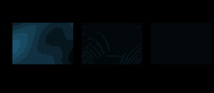
A raster warped to Lambert azimuthal equal-area and back, nearest against bilinear. The left panel is the field the raster carries — a smooth analytic function, so that the error of an interpolation is the interpolation's error and not a photograph's history. The other panels are what is left after warping into Lambert azimuthal equal-area and back to Equirectangular, shown as the difference from the original at six times the contrast. Nothing moved: the coordinates go through the maps exactly. What is lost is that a target pixel's centre does not fall on a source pixel's centre, so a value has to be invented for it. Bilinear is closer to the field — RMS 0.0022 against 0.0212 — and has given up 0.63 per cent of its variance to get there. The panels are drawn at 48 by 32 cells; the measurement is made at the same resolution.

Reprojecting a raster invents values

Moving a picture from one projection to another moves no coordinate — the maps are exact both ways. What is lost is that a target cell's centre does not land on a source cell's centre, so a value has to be made up for it, and the making-up has an order of convergence: 1.00 for nearest, 1.98 for bilinear, 2.93 for a cubic, measured by refining the grid.

applied · Dataset
Three implementations of one projection, and three different distortions. The spread in angular deformation between linear, Catmull–Rom and Aitken interpolations of Robinson's own table, at 60° of longitude. It is exactly zero at every fifth degree, because all three pass through the tabulated rows, and it is not zero anywhere else: 37 of 87 latitudes differ by more than half a degree and the worst is 8.42°. The graticules the three draw differ by 4.2 parts per thousand of the map's own span, which is under the width of a printed line.

A projection defined by a table has an interpolation in it

One member of this library has no formula: Robinson set nineteen pairs of numbers by eye and the table is the definition. Three published interpolations of it draw graticules that differ by four parts in a thousand of the map's span and report angular deformations that differ by 8.4 degrees.

families · Families
The same kernels, across an edge. Each kernel measured over the same five rasters as the smooth measurement, on a field that carries a step across a tilted line instead of a smooth function. The solid lines are the edge and the faint ones the smooth field. The orders on the smooth field are nearest 1.00, bilinear 1.98, cubic 2.93; across the edge they are nearest 0.78, bilinear 0.58, cubic 0.60 — within a factor of 1.33 of one another, and the fastest of them belongs to nearest-neighbour, which does no interpolating at all. The ranking a smooth field establishes does not survive a discontinuity, and a real raster is mostly edges.

An edge has no order of convergence

On a smooth field the three resampling kernels converge at orders 1, 2 and 3 and the choice is obvious. Across a discontinuity they converge at 0.78, 0.58 and 0.60 — within a factor of 1.4 of each other, in an order that puts nearest-neighbour first, and a real raster is mostly edges.

applied · Dataset
One field, one round trip between two cell schemes. Left: a stated field binned into an equal-angle grid of 36 by 18 cells. Right: the same field after being rebinned into an equal-area grid of 30 by 15 offset by six degrees of longitude, and rebinned back. Every step is exact area-weighted averaging, the total is preserved to 2 × 10⁻¹⁶, and the root-mean-square difference between the two pictures is 0.144 on a field whose own standard deviation is 0.370.

The same data on two grids

Five essays have addressed, queried and ordered cells within one scheme and nobody has moved a number between two. Doing it exactly — area-weighted, both directions — preserves the total to 2 × 10⁻¹⁶ and loses 39 per cent of the field's own standard deviation in a single round trip; six round trips leave 23 per cent of its variance. The quantity that would reveal the damage is the one that never moves.

applied · Cells
The piece two schemes share, clipped rather than assumed. A cell of a gnomonic cube, whose four edges are great-circle arcs because a straight line on a gnomonic face is one, against a cell of a longitude–latitude grid, whose north and south edges are parallels and are not. Their overlap is neither a rectangle nor a spherical polygon of any standard kind, and it is 5965687 km² of the cube cell's 5965687 km² — 100.0 per cent. Computing it needs the arc of one boundary intersected with the plane of the other, which is three equations and two roots, and it is exact.

Cells that are rectangles in no coordinate

The previous rung measured what moving a field between two cell schemes costs, and did it between two schemes whose cells are longitude–latitude rectangles — which is what made every overlap a rectangle with a closed-form area. The schemes anybody actually argues about have cells that are rectangles in no coordinate, and their overlaps have to be clipped.

applied · Cells
Two source geometries of 96 cells each, rebinned to the same three targets. Both curves start from a source of 96 cells and rebin to targets of 32, 128, 512 cells, so the count ratio is identical along them and the only difference is the shape of the source cells: gnomonic squares on a cube against rectangles in longitude and latitude. The ratio dominates — both curves fall by more than half across the range — and the shapes still separate by 25 points at the middle target. The cube loses less, because its cells are all much the same size and the lon/lat source's collapse towards the poles.

The same number of cells, in two shapes

Moving a field between two cell schemes loses 18 per cent of it per cell in one geometry and 39 in another, and the earlier measurement could not say whether that was the shape of the cells or the ratio of their sizes, because changing the schemes changed both. Holding the counts settles it: the count ratio decides most of the loss, and the shape is still worth a quarter of the field.

applied · Cells
Two compromises along one path, and they do not agree. The angular deformation and the flexion of every blend between Mercator and Lambert cylindrical, each divided by the straight line between the two parents' own values. A value of one means the blend is exactly the average of the two errors and has bought nothing. The angular deformation dips to 0.649 at a weight of 0.13; the flexion dips only to 0.955, and it does so at 0.50. Anybody choosing a compromise is choosing a weight, and the two orders want different ones.

The best compromise for angle is not the best for bending

Every compromise projection in the library is an average of two others, and averaging is a first-order operation — so the second derivative was never part of the bargain. Swept along five ordinary blend paths, the weight that minimises angular deformation and the weight that minimises flexion are between a quarter and a half of the axis apart, and how much a compromise buys at one order predicts nothing about the other.

distortion · Flexion
The doubling ladder is the one sequence that cannot see it. The largest departure of a small circle from its own indicatrix that a grid of n latitudes over 10° to 70° north finds on the Robinson projection. The filled marks are 4, 8, 16, 32, 64 and 128 — the doubling ladder every convergence study runs — and they rise smoothly to about 4.66e-4 with the increments halving, which is what a convergent first-order sequence looks like. The open marks are grids whose samples land on the projection's five-degree table entries. They report 1.28e-2, twenty-seven times higher, and whether a grid does that is decided by whether n is a multiple of four.

A refinement that stops moving

Doubling the sample and watching the answer settle is how every quadrature in every field is checked. On the Robinson projection the doubling ladder — 4, 8, 16, 32, 64, 128 — converges beautifully, with its increments halving at every step, on a limit that is wrong by a factor of twenty-seven. Whether a grid finds the answer is decided by whether n is a multiple of four.

distortion · Sampling

Named alongside it

The objects these essays reach for when they reach for this one.

ToleranceVerificationAggregationConservationConvergence orderDiscrete global gridResamplingRobinsonAngular deformationAreaCell systemClipping

All concepts